AI and Deep Learning

In this course, you'll build AI projects that can answer simple visual questions: Is my hand showing thumbs-up or thumbs-down?

• Does my face appear happy or sad?
• How many fingers am I holding up?
• Where's my nose?

Although these questions are easy for any human child to answer, interpreting images with computer vision requires a complex computer model that can be tuned to find the answer in a number of scenarios. For example, a thumbs-up hand signal may be at various angles and distances from the camera, it may be held before a variety of backgrounds, it could be from a variety of different hands, and so on, but it is still a thumbs-up hand signal. An effective AI model must be able to generalize across these scenarios, and even predict the correct answer with new data.

AI and Deep Learning

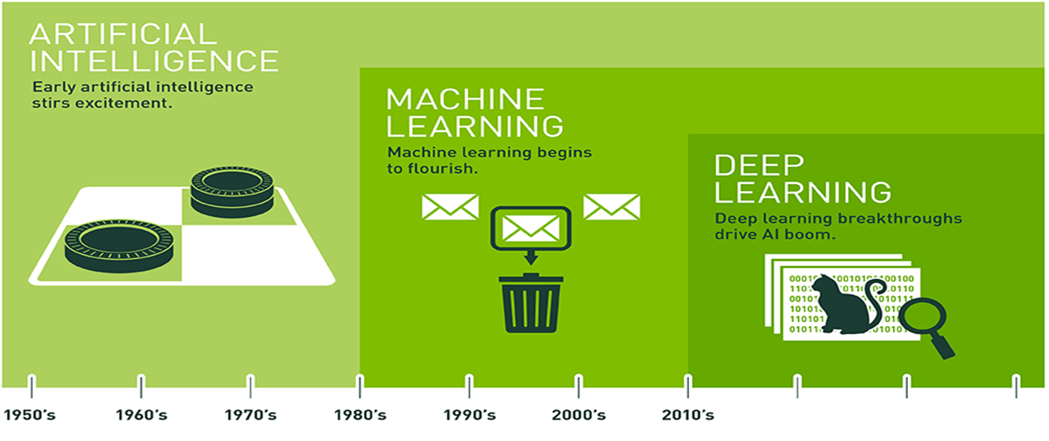
As humans, we generalize what we see based on our experience. In a similar way, we can use a branch of AI called Machine Learning to generalize and classify images based on experience in the form of lots of example data. In particular, we will use deep neural network models, or Deep Learning to recognize relevant patterns in an image dataset, and ultimately match new images to correct answers.

Deep Learning Models

A Deep Learning model consists of a neural network with internal parameters, or weights, configured to map inputs to outputs. In Image Classification, the inputs are the pixels from a camera image and the outputs are the possible categories, or classes that the model is trained to recognize. The choices might be 1000 different objects, or only two. Multiple labeled examples must be provided to the model over and over to train it to recognize the images. Once the model is trained, it can be run on live data and provide results in real time. This is called inference.

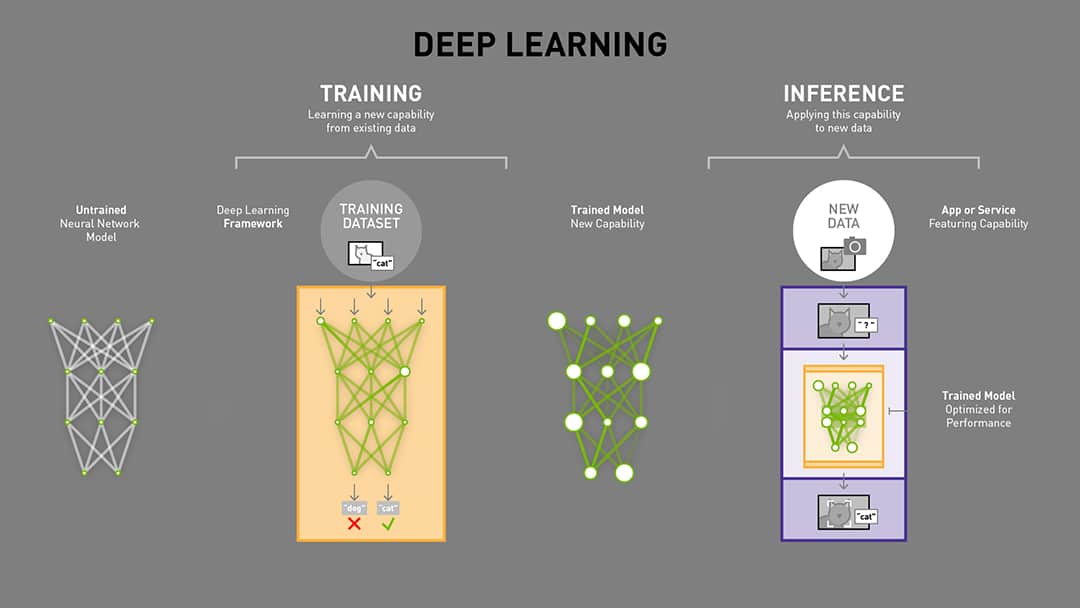
Before training, the model cannot accurately determine the correct class from an image input, because the weights are wrong. Labeled examples of images are iteratively submitted to the network with a learning algorithm. If the network gets the "wrong" answer (the label doesn't match), the learning algorithm adjusts the weights a little bit. Over many computationally intensive iterations, the accuracy improves to the point that the model can reliably determine the class for an input image.

As you will discover, the data that is input is one of the keys to a good model, i.e. one that generalizes well regardless of the background, angle, or other "noisy" aspect of the image presented. Additional passes through the data set, or epochs can also improve the model's performance.

Convolutional Neural Networks (CNNs)

Deep learning relies on Convolutional Neural Network (CNN) models to transform images into predicted classifications. A CNN is a class of artificial neural network that uses convolutional layers to filter inputs for useful information, and is the preferred network for image applications.

Artificial Neural Network

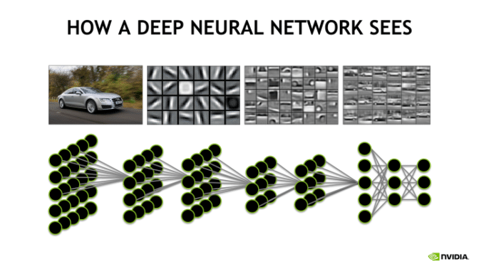
An artificial neural network is a biologically inspired computational model that is patterned after the network of neurons present in the human brain. At each layer, the network transforms input data by applying a nonlinear function to a weighted sum of the inputs. The intermediate outputs of one layer, called features, are used as the input into the next layer. The neural network, through repeated transformations, learns multiple layers of nonlinear features (like edges and shapes), which it then combines in a final layer to create a prediction (of more complex objects).

The neural network learns by generating an error signal that measures the difference between the predictions of the network and the desired values and then using this error signal to change the weights (or parameters) so that predictions get more accurate.

Convolutions

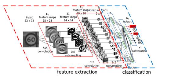
The convolution operation specific to CNNs combines the input data (feature map) from one layer with a convolution kernel (filter) to form a transformed feature map for the next layer. CNNs for image classification are generally composed of an input layer (the image), a series of hidden layers for feature extraction (the convolutions), and a fully connected output layer (the classification).

For example, the below image by Maurice Peemen shows: An input image of a traffic sign is filtered by 4 5x5 convolutional kernels which create 4 feature maps, these feature maps are subsampled by max pooling. The next layer applies 10 5x5 convolutional kernels to these subsampled images and again we pool the feature maps. The final layer is a fully connected layer where all generated features are combined and used in the classifier (essentially logistic regression).

As it is trained, the CNN adjusts automatically to find the most relevant features based on its classification requirements. For example, a CNN would filter information about the shape of an object when confronted with a general object recognition task but would extract the color of the bird when faced with a bird recognition task. This is based on the CNN's recognition through training that different classes of objects have different shapes but that different types of birds are more likely to differ in color than in shape.

ResNet-18

There are a number of world-class CNN architectures available to application developers for image classification and image regression. PyTorch and other frameworks include access to pretrained models from past winners of the famous Imagenet Large Scale Visual Recognition Challenge (ILSVRC), where researchers compete to correctly classify and detect objects and scenes with computer vision algorithms. In 2015, ResNet swept the awards in image classification, detection, and localization. We'll be using the smallest version of ResNet in our projects: ResNet-18.

Transfer Learning

PyTorch includes a pre-trained ResNet-18 model that was trained on the ImageNet 2012 classification dataset, which consists of 1000 classes. In other words, the model can recognize 1000 different objects already!

Within the trained neural network are layers that find outlines, curves, lines, and other identifying features of an image. Important image features that were already learned in the original training of the model are now re-usable for our own classification task.

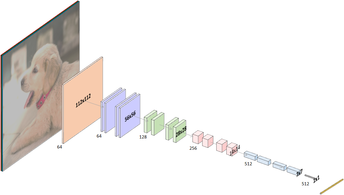
We will adapt it for our projects, which all include less than 10 different classes, by modifying the last neural network layer of the 18 that make up the ResNet-18 model. The last layer for ResNet-18 is a fully connected (fc) layer, pooled and flattened to 512 inputs, each connected to the 1000 possible output classes. We will replace the (512,1000) layer with one matching our classes. If we only need three classes, for example, this final layer will become (512, 3), where each of the 512 inputs is fully connected to each one of the 3 output classes.

You will still need to train the network to recognize those three classes using images you collect, but since the network has already learned to recognize features common to most objects, training is already part-way done. The previous training can be reused, or "transferred" to your new projects.

Accelerating CNNs using GPUs

The extensive calculations required for training CNN models and running inference through trained CNN models can be quite large in number, requiring intensive compute resources and time. Deep learning frameworks such as Caffe, TensorFlow, and PyTorch, are optimized to run faster on GPUs. The frameworks take advantage of the parallel processing capabilities of a GPU if it is present, speeding up training and inference tasks.

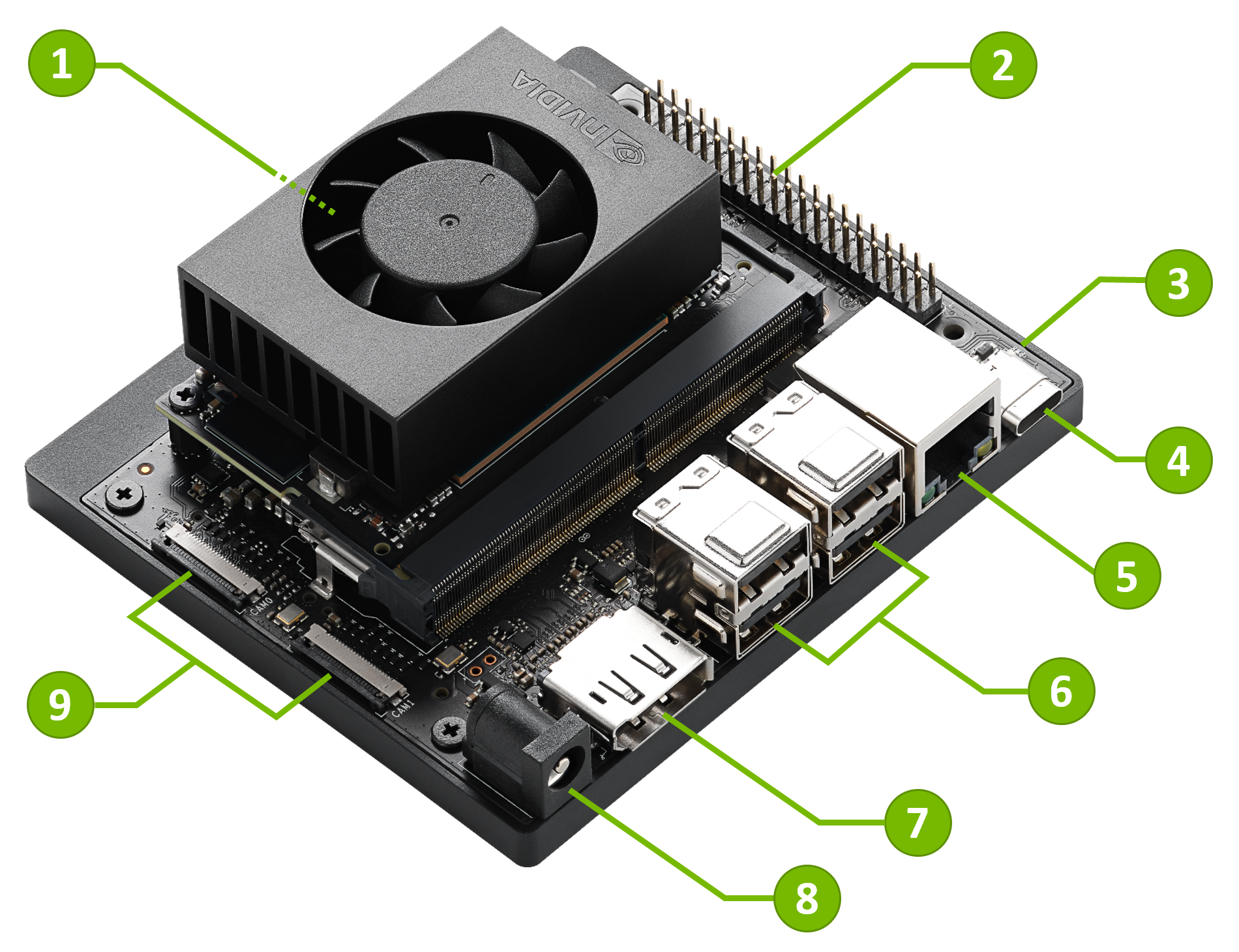
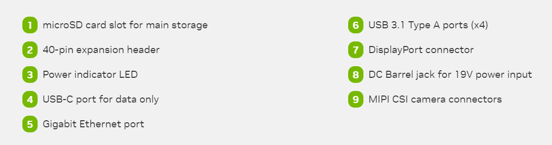
The Jetson Orin Nano includes 1024 NVIDIA CUDA Cores and 32 Tensor Cores GPU. Since it can run the full training frameworks, it is also able to re-train networks with transfer learning, a capability you will use in the projects for this lab. Jetson Orin Nano sets a new standard for creating entry-level AI-powered robots, smart drones, and intelligent vision systems.

Interactive Regression Tool

This notebook is an interactive data collection, training, and testing tool, based on NVIDIA course.

Camera

First, create your camera and set it to running. Uncomment the appropriate camera selection lines, depending on which type of camera you're using (USB or CSI). This cell may take several seconds to execute.

There can only be one instance of CSICamera or USBCamera at a time. Before starting a new project and creating a new camera instance, you must first release the existing one. To do so, shut down the notebook's kernel from the JupyterLab pull-down menu: Kernel->Shutdown Kernel, then restart it with Kernel->Restart Kernel.

sudo systemctl restart nvargus-daemon is included to then force a reset of the camera daemon.

# Check device number
!ls -ltrh /dev/video*

# USB Camera (Logitech C270 webcam)
#from jetcam.usb_camera import USBCamera
#camera = USBCamera(width=224, height=224, capture_device=0) # confirm the capture_device number

# CSI Camera
from jetcam.csi_camera import CSICamera
# camera = CSICamera(width=480, height=480, capture_width=1920, capture_height=1080, capture_fps=30)
#camera = CSICamera(capture_device=1, flip_method=2, width=224, height=224, capture_width=1920, capture_height=1080, capture_fps=30)
camera = CSICamera(capture_device=0, width=224, height=224, capture_width=1920, capture_height=1080, capture_fps=30)

camera.running = True
print("camera created")

crw-rw---- 1 root video 81, 0 Sep 30 04:11 /dev/video0
GST_ARGUS: Creating output stream
CONSUMER: Waiting until producer is connected...
GST_ARGUS: Available Sensor modes :
GST_ARGUS: 3280 x 2464 FR = 21.000000 fps Duration = 47619048 ; Analog Gain range min 1.000000, max 10.625000; Exposure Range min 13000, max 683709000;

GST_ARGUS: 3280 x 1848 FR = 28.000001 fps Duration = 35714284 ; Analog Gain range min 1.000000, max 10.625000; Exposure Range min 13000, max 683709000;

GST_ARGUS: 1920 x 1080 FR = 29.999999 fps Duration = 33333334 ; Analog Gain range min 1.000000, max 10.625000; Exposure Range min 13000, max 683709000;

GST_ARGUS: 1640 x 1232 FR = 29.999999 fps Duration = 33333334 ; Analog Gain range min 1.000000, max 10.625000; Exposure Range min 13000, max 683709000;

GST_ARGUS: 1280 x 720 FR = 59.999999 fps Duration = 16666667 ; Analog Gain range min 1.000000, max 10.625000; Exposure Range min 13000, max 683709000;

GST_ARGUS: Running with following settings:
   Camera index = 0 
   Camera mode  = 2 
   Output Stream W = 1920 H = 1080 
   seconds to Run    = 0 
   Frame Rate = 29.999999 
GST_ARGUS: Setup Complete, Starting captures for 0 seconds
GST_ARGUS: Starting repeat capture requests.
CONSUMER: Producer has connected; continuing.
camera created

[ WARN:0@0.744] global cap_gstreamer.cpp:1728 open OpenCV | GStreamer warning: Cannot query video position: status=0, value=-1, duration=-1

Regression

Regression is a core technique in machine learning used to predict continuous values based on input data. Unlike classification, which assigns data to discrete categories, regression models learn to estimate numerical outputs—making them ideal for tasks involving tracking, positioning, or forecasting.
In this experiment, we will explore how regression can be applied to real-time object tracking. Using a camera, the system will attempt to follow a specific point on the human body, such as the hand or nose, by predicting its position frame by frame. This technique is highly relevant in applications like autonomous vehicles or robotic systems, where accurately following a moving target is essential for navigation, interaction, and control.

Task

Next, define your project TASK and what CATEGORIES of data you will collect. You may optionally define space for multiple DATASETS with names of your choosing.

Uncomment/edit the associated lines for the XY regression task you're building and execute the cell. This cell should only take a few seconds to execute.

import torchvision.transforms as transforms
from dataset import XYDataset

TASK = 'body'
# TASK = 'diy'

CATEGORIES = ['hand','nose', 'left_eye', 'right_eye']
# CATEGORIES = [ 'diy_1', 'diy_2', 'diy_3']

DATASETS = ['A', 'B']
# DATASETS = ['A', 'B', 'C']

TRANSFORMS = transforms.Compose([
    transforms.ColorJitter(0.2, 0.2, 0.2, 0.2),
    transforms.Resize((224, 224)),
    transforms.ToTensor(),
    transforms.Normalize([0.485, 0.456, 0.406], [0.229, 0.224, 0.225])
])

datasets = {}
for name in DATASETS:
    datasets[name] = XYDataset(TASK + '_' + name, CATEGORIES, TRANSFORMS)
    
print("{} task with {} categories defined".format(TASK, CATEGORIES))

body task with ['hand', 'nose', 'left_eye', 'right_eye'] categories defined

Data Collection

In this part of the experiment, you will capture an image using the camera and manually select the point you wish to track—such as the hand or nose—by clicking on it. The system will record the coordinates (x, y) of your click along with the image. This labeled data will then be used to train a regression model that learns to predict the position of the selected point in future frames.
Execute the cell below to create the data collection tool widget. This cell should only take a few seconds to execute.

import cv2
import ipywidgets
import traitlets
from IPython.display import display
from jetcam.utils import bgr8_to_jpeg
from ipyevents import Event

# initialize active dataset
dataset = datasets[DATASETS[0]]

# unobserve all callbacks from camera in case we are running this cell for second time
camera.unobserve_all()

# create image preview
camera_widget = ipywidgets.Image(width=camera.width, height=camera.height)
with open("./images/ready_img.jpg", "rb") as file:
    default_image = file.read()
snapshot_widget = ipywidgets.Image(value=default_image, width=camera.width, height=camera.height)
traitlets.dlink((camera, 'value'), (camera_widget, 'value'), transform=bgr8_to_jpeg)

# create event for image click
im_events = Event(source=camera_widget, watched_events=['click'], wait=500, throttle_or_debounce='debounce')

#  prevent the image from being dragged if a user clicks
no_drag = Event(source=camera_widget, watched_events=['dragstart'], prevent_default_action = True)

# create widgets (Add a widget for dropdown menu of the datasets and for categories) ...TO DO
dataset_widget = ipywidgets.Dropdown(options=DATASETS, description='dataset')
category_widget = ipywidgets.Dropdown(options=dataset.categories, description='category')

# create widgets for count and saving button
count_widget = ipywidgets.IntText(description='count')

# manually update counts at initialization
count_widget.value = dataset.get_count(category_widget.value)

# sets the active dataset
def set_dataset(change):
    global dataset
    dataset = datasets[change['new']]
    count_widget.value = dataset.get_count(category_widget.value)
dataset_widget.observe(set_dataset, names='value')

# update counts when we select a new category
def update_counts(change):
    count_widget.value = dataset.get_count(change['new'])
category_widget.observe(update_counts, names='value')

# save image for category and update counts
def save_snapshot(event):
    x = event['dataX']
    y = event['dataY']
    
    if x != 0 and y != 0:
        #save to disk
        dataset.save_entry(category_widget.value, camera.value, x, y)
        
        # display saved snapshot
        snapshot = camera.value.copy()
        snapshot = cv2.circle(snapshot, (x, y), 8, (0, 255, 0), 3)
        snapshot_widget.value = bgr8_to_jpeg(snapshot)
        count_widget.value = dataset.get_count(category_widget.value)
        
im_events.on_dom_event(save_snapshot)

data_collection_widget = ipywidgets.VBox([
    ipywidgets.HBox([camera_widget, snapshot_widget]),
    dataset_widget,
    category_widget,
    count_widget
])

display(data_collection_widget)
print("data_collection_widget created")

VBox(children=(HBox(children=(Image(value=b'\xff\xd8\xff\xe0\x00\x10JFIF\x00\x01\x01\x00\x00\x01\x00\x01\x00\x…

data_collection_widget created

Now, let's close the camera conneciton properly so that we can use the camera later.

camera.unobserve_all()

Visualization utilities

Execute the cell below to enable live plotting.

from bokeh.io import push_notebook, show, output_notebook
from bokeh.layouts import row
from bokeh.plotting import figure
from bokeh.models import ColumnDataSource
from bokeh.models.tickers import SingleIntervalTicker
output_notebook()

colors = ['#1f77b4', '#ff7f0e', '#2ca02c', '#d62728']

p1 = figure(title="Loss", x_axis_label="Epoch", height=300, width=360)

source1 = ColumnDataSource(data={'epochs': [], 'trainlosses': []})

#r = p1.multi_line(ys=['trainlosses', 'testlosses'], xs='epochs', color=colors, alpha=0.8, legend_label=['Training','Test'], source=source)
r1 = p1.line(x='epochs', y='trainlosses', line_width=2, color=colors[0], alpha=0.8, legend_label="Train", source=source1)


p1.legend.location = "top_right"
p1.legend.click_policy="hide"

Loading BokehJS ...

Model

Define the neural network

Now, we define the neural network we'll be training. The torchvision package provides a collection of pre-trained models that we can use.

In a process called transfer learning, we can repurpose a pre-trained model (trained on millions of images) for a new task that has possibly much less data available.

Important features that were learned in the original training of the pre-trained model are re-usable for the new task. We'll use the resnet18 model.

import torch
import torchvision
import time
import torch.nn.functional as F
from torch import nn

# RESNET 18
model = torchvision.models.resnet18(weights='IMAGENET1K_V1')

The resnet18 model was originally trained for a dataset that had 1000 class labels, but our dataset only has nubmer of class labels based on categories! We'll replace the final layer with a new, untrained layer that has only two outputs.

output_dim = 2 * len(dataset.categories)  # x, y coordinate for each category

model.fc = torch.nn.Linear(512, output_dim)

Finally, we transfer our model for execution on the GPU

device = torch.device('cuda')
model = model.to(device)

torchvision backage has Other pre-trained models that could be selected and tested

# ALEXNET
# model = torchvision.models.alexnet(pretrained=True).to(device)
# model.classifier[-1] = torch.nn.Linear(4096, len(dataset.categories))

# SQUEEZENET 
# model = torchvision.models.squeezenet1_1(pretrained=True).to(device)
# model.classifier[1] = torch.nn.Conv2d(512, len(dataset.categories), kernel_size=1)
# model.num_classes = len(dataset.categories)


# RESNET 34
# model = torchvision.models.resnet34(pretrained=True).to(device)
# model.fc = torch.nn.Linear(512, len(dataset.categories))

Create widget to save the saved trained model and widget to load previous saved model

model_save_button = ipywidgets.Button(description='save model')
model_load_button = ipywidgets.Button(description='load model')
model_path_widget = ipywidgets.Text(description='model path', value='my_model.pth')

def load_model(c):
    model.load_state_dict(torch.load(model_path_widget.value))
model_load_button.on_click(load_model)
    
def save_model(c):
    torch.save(model.state_dict(), model_path_widget.value)
model_save_button.on_click(save_model)

model_widget = ipywidgets.VBox([
    model_path_widget,
    ipywidgets.HBox([model_load_button, model_save_button])
])

print("model configured and model_widget created")

model configured and model_widget created

Training and Evaluation

In this section, we will train a regression model using the labeled data collected earlier. The training process involves feeding batches of images and their corresponding coordinates into the model, allowing it to learn the relationship between visual input and target position.
You can customize key training parameters such as batch size, optimizer, and number of epochs using interactive widgets. As the model trains, a dynamic plot will display the loss values in real time, helping you monitor the model’s learning progress and convergence. This visualization provides valuable insight into how well the model is adapting to the data and whether adjustments are needed.
Execute the following cell to define the trainer, and the widget to control it.

BATCH_SIZE = 8

optimizer = torch.optim.Adam(model.parameters())
# optimizer = torch.optim.SGD(model.parameters(), lr=1e-3, momentum=0.9)

# Handle to plot Loss and Accuracy Graph
#handle = show(row(p1, p2), notebook_handle=True)
handle = show(p1, notebook_handle=True)

epochs_widget = ipywidgets.IntText(description='epochs', value=1)
eval_button = ipywidgets.Button(description='evaluate')
train_button = ipywidgets.Button(description='train')
loss_widget = ipywidgets.FloatText(description='loss')
progress_widget = ipywidgets.FloatProgress(min=0.0, max=1.0, description='progress')

def train_eval(is_training):
    global BATCH_SIZE, LEARNING_RATE, MOMENTUM, model, dataset, optimizer, eval_button, train_button, accuracy_widget, loss_widget, progress_widget
    
    try:
        train_loader = torch.utils.data.DataLoader(
            dataset,
            batch_size=BATCH_SIZE,
            shuffle=True
        )

        
        train_button.disabled = True
        eval_button.disabled = True
        time.sleep(1)

        if is_training:
            model = model.train()
        else:
            model = model.eval()

            
        epochs = epochs_widget.value
        
        while epochs_widget.value > 0:
            i = 0
            sum_loss = 0.0
            error_count = 0.0
            for images, category_idx, xy in iter(train_loader):
                # send data to device
                images = images.to(device)
                xy = xy.to(device)

                if is_training:
                    # zero gradients of parameters
                    optimizer.zero_grad()

                # execute model to get outputs
                outputs = model(images)

                # compute MSE loss over x, y coordinates for associated categories
                loss = 0.0
                for batch_idx, cat_idx in enumerate(list(category_idx.flatten())):
                    loss += torch.mean((outputs[batch_idx][2 * cat_idx:2 * cat_idx+2] - xy[batch_idx])**2)
                loss /= len(category_idx)

                if is_training:
                    # run backpropogation to accumulate gradients
                    loss.backward()

                    # step optimizer to adjust parameters
                    optimizer.step()

                # increment progress
                count = len(category_idx.flatten())
                i += count
                sum_loss += float(loss)
                progress_widget.value = i / len(dataset)
                loss_widget.value = sum_loss / i

                new_data1 = {'epochs': [epochs-epochs_widget.value+progress_widget.value],
                             'trainlosses': [float(loss_widget.value)]}
                source1.stream(new_data1)
                
                push_notebook(handle=handle)
                
            if is_training:
                epochs_widget.value = epochs_widget.value - 1
            else:
                break
    except e:
        pass
    model = model.eval()

    train_button.disabled = False
    eval_button.disabled = False
    
    
train_button.on_click(lambda c: train_eval(is_training=True))
eval_button.on_click(lambda c: train_eval(is_training=False))
    
train_eval_widget = ipywidgets.VBox([
    epochs_widget,
    progress_widget,
    loss_widget,
    ipywidgets.HBox([train_button, eval_button])
])

display(train_eval_widget)
print("trainer configured and train_eval_widget created")

VBox(children=(IntText(value=1, description='epochs'), FloatProgress(value=0.0, description='progress', max=1.…

trainer configured and train_eval_widget created

Live Execution

In this final stage of the experiment, the trained regression model will be deployed in real time. A camera feed will continuously track the selected target—such as a hand or nose—and display a dot that follows its predicted position on the screen. This live demonstration showcases how regression can be used for dynamic object tracking, a technique widely applicable in autonomous systems and robotics for tasks like gesture control, human-following, and interactive navigation.
Execute the cell below to set up the live execution widget. This cell should only take a few seconds to execute.

import threading
import time
from utils import preprocess
import torch.nn.functional as F

state_widget = ipywidgets.ToggleButtons(options=['stop', 'live'], description='state', value='stop')
with open("./images/ready_img.jpg", "rb") as file:
    default_image = file.read()
prediction_widget = ipywidgets.Image(format='jpeg', width=camera.width, height=camera.height, value=default_image)

def live(state_widget, model, camera, prediction_widget):
    global dataset
    while state_widget.value == 'live':
        image = camera.value
        preprocessed = preprocess(image)
        output = model(preprocessed).detach().cpu().numpy().flatten()
        category_index = dataset.categories.index(category_widget.value)
        x = output[2 * category_index]
        y = output[2 * category_index + 1]
        
        x = int(camera.width * (x / 2.0 + 0.5))
        y = int(camera.height * (y / 2.0 + 0.5))
        
        prediction = image.copy()
        prediction = cv2.circle(prediction, (x, y), 8, (255, 0, 0), 3)
        prediction_widget.value = bgr8_to_jpeg(prediction)
            
def start_live(change):
    if change['new'] == 'live':
        execute_thread = threading.Thread(target=live, args=(state_widget, model, camera, prediction_widget))
        execute_thread.start()

state_widget.observe(start_live, names='value')

live_execution_widget = ipywidgets.VBox([
    prediction_widget,
    state_widget
])

display(live_execution_widget)
print("live_execution_widget created")

VBox(children=(Image(value=b'\xff\xd8\xff\xe0\x00\x10JFIF\x00\x01\x01\x01\x00\xf0\x00\xf0\x00\x00\xff\xdb\x00C…

live_execution_widget created