Inference and Validation

Now that you have a trained network, you can use it for making predictions. This is typically called inference, a term borrowed from statistics. However, neural networks have a tendency to perform too well on the training data and aren't able to generalize to data that hasn't been seen before. This is called overfitting and it impairs inference performance. To test for overfitting while training, we measure the performance on data not in the training set called the validation set. We avoid overfitting through regularization such as dropout while monitoring the validation performance during training. In this notebook, I'll show you how to do this in PyTorch.

As usual, let's start by loading the dataset through torchvision. You'll learn more about torchvision and loading data in a later part. This time we'll be taking advantage of the test set which you can get by setting train=False here:

testset = datasets.FashionMNIST('~/.pytorch/F_MNIST_data/', download=True, train=False, transform=transform)  # Download/load Fashion-MNIST test data

The test set contains images just like the training set. Typically you'll see 10-20% of the original dataset held out for testing and validation with the rest being used for training.

import torch  # Import PyTorch library
from torchvision import datasets, transforms  # Import datasets and image transforms

# Define a transform to normalize the data
transform = transforms.Compose([transforms.ToTensor(),  # Define transform: convert to tensor
                                transforms.Normalize((0.5,), (0.5,))])
# Download and load the training data
trainset = datasets.FashionMNIST('~/.pytorch/F_MNIST_data/', download=True, train=True, transform=transform)  # Download/load Fashion-MNIST training data
trainloader = torch.utils.data.DataLoader(trainset, batch_size=64, shuffle=True)  # Create training data loader

# Download and load the test data
testset = datasets.FashionMNIST('~/.pytorch/F_MNIST_data/', download=True, train=False, transform=transform)  # Download/load Fashion-MNIST test data
testloader = torch.utils.data.DataLoader(testset, batch_size=64, shuffle=True)  # Create test data loader

Here I'll create a model like normal, using the same one from my solution for part 4.

from torch import nn, optim
import torch.nn.functional as F  # Import functional API (F.relu, etc.)

class Classifier(nn.Module):  # Define neural network class
    def __init__(self):  # Initialize network layers
        super().__init__()  # Initialize parent class
        self.fc1 = nn.Linear(784, 256)  # First fully connected layer
        self.fc2 = nn.Linear(256, 128)  # Second fully connected layer
        self.fc3 = nn.Linear(128, 64)  # Third fully connected layer
        self.fc4 = nn.Linear(64, 10)  # Output layer
        
    def forward(self, x):
        # make sure input tensor is flattened
        x = x.view(x.shape[0], -1)  # Flatten: (batch, 1, 28, 28) -> (batch, 784)
        
        x = F.relu(self.fc1(x))  # FC1 -> ReLU activation
        x = F.relu(self.fc2(x))  # FC2 -> ReLU activation
        x = F.relu(self.fc3(x))  # FC3 -> ReLU activation
        x = F.log_softmax(self.fc4(x), dim=1)  # FC4 -> LogSoftmax output
        
        return x  # Return output tensor

The goal of validation is to measure the model's performance on data that isn't part of the training set. Performance here is up to the developer to define though. Typically this is just accuracy, the percentage of classes the network predicted correctly. Other options are precision and recall) and top-5 error rate. We'll focus on accuracy here. First I'll do a forward pass with one batch from the test set.

model = Classifier()  # Instantiate the Classifier model

images, labels = next(iter(testloader))
# Get the class probabilities
ps = torch.exp(model(images))
# Make sure the shape is appropriate, we should get 10 class probabilities for 64 examples
print(ps.shape)

With the probabilities, we can get the most likely class using the ps.topk method. This returns the $k$ highest values. Since we just want the most likely class, we can use ps.topk(1). This returns a tuple of the top-$k$ values and the top-$k$ indices. If the highest value is the fifth element, we'll get back 4 as the index.

top_p, top_class = ps.topk(1, dim=1)  # Get top prediction
# Look at the most likely classes for the first 10 examples
print(top_class[:10,:])

Now we can check if the predicted classes match the labels. This is simple to do by equating top_class and labels, but we have to be careful of the shapes. Here top_class is a 2D tensor with shape (64, 1) while labels is 1D with shape (64). To get the equality to work out the way we want, top_class and labels must have the same shape.

If we do

equals = top_class == labels

equals will have shape (64, 64), try it yourself. What it's doing is comparing the one element in each row of top_class with each element in labels which returns 64 True/False boolean values for each row.

equals = top_class == labels.view(*top_class.shape)  # Compare predictions to actual labels

Now we need to calculate the percentage of correct predictions. equals has binary values, either 0 or 1. This means that if we just sum up all the values and divide by the number of values, we get the percentage of correct predictions. This is the same operation as taking the mean, so we can get the accuracy with a call to torch.mean. If only it was that simple. If you try torch.mean(equals), you'll get an error

RuntimeError: mean is not implemented for type torch.ByteTensor

This happens because equals has type torch.ByteTensor but torch.mean isn't implemented for tensors with that type. So we'll need to convert equals to a float tensor. Note that when we take torch.mean it returns a scalar tensor, to get the actual value as a float we'll need to do accuracy.item().

accuracy = torch.mean(equals.type(torch.FloatTensor))
print(f'Accuracy: {accuracy.item()*100}%')

The network is untrained so it's making random guesses and we should see an accuracy around 10%. Now let's train our network and include our validation pass so we can measure how well the network is performing on the test set. Since we're not updating our parameters in the validation pass, we can speed up our code by turning off gradients using torch.no_grad():

# turn off gradients
with torch.no_grad():  # Disable gradient computation
    # validation pass here
    for images, labels in testloader:  # Loop through test batches
        ...

Exercise: Implement the validation loop below and print out the total accuracy after the loop. You can largely copy and paste the code from above, but I suggest typing it in because writing it out yourself is essential for building the skill. In general you'll always learn more by typing it rather than copy-pasting. You should be able to get an accuracy above 80%.

model = Classifier()
criterion = nn.NLLLoss()  # Negative log-likelihood loss
optimizer = optim.Adam(model.parameters(), lr=0.003)  # Adam optimizer

epochs = 15  # Number of training epochs

train_losses, test_losses = [], []
for e in range(epochs):  # Loop through each epoch
    tot_train_loss = 0
    for images, labels in trainloader:
        optimizer.zero_grad()  # Clear previous gradients
        
        log_ps = model(images)
        loss = criterion(log_ps, labels)  # Calculate loss
        tot_train_loss += loss.item()
        
        loss.backward()  # Backpropagate gradients
        optimizer.step()  # Update model weights
    else:  # After epoch completes
        tot_test_loss = 0
        test_correct = 0  # Number of correct predictions on the test set

        ## TODO: Implement the validation pass and print out the validation accuracy
        # Turn off gradients for validation, saves memory and computations
        with torch.no_grad():  # Disable gradient computation
            for images, labels in testloader:  # Loop through test batches
                log_ps = 
                loss = 
                tot_test_loss += loss.item()

                ps = 
                top_p, top_class = 
                equals = 
                test_correct += equals.sum().item()

        # Get mean loss to enable comparison between train and test sets
        train_loss = tot_train_loss / len(trainloader.dataset)
        test_loss = tot_test_loss / len(testloader.dataset)

        # At completion of epoch
        train_losses.append(train_loss)  # Save train loss
        test_losses.append(test_loss)  # Save test loss

        print("Epoch: {}/{}.. ".format(e+1, epochs),
              "Training Loss: {:.3f}.. ".format(train_loss),
              "Test Loss: {:.3f}.. ".format(test_loss),
              "Test Accuracy: {:.3f}".format(test_correct / len(testloader.dataset)))

%matplotlib inline  # Enable inline plotting in notebook
%config InlineBackend.figure_format = 'retina'

import matplotlib.pyplot as plt  # Import matplotlib for visualization

plt.plot(train_losses, label='Training loss')  # Plot training loss curve
plt.plot(test_losses, label='Validation loss')  # Plot test/validation loss curve
plt.legend(frameon=False)  # Add legend to plot

Overfitting

If we look at the training and validation losses as we train the network, we can see a phenomenon known as overfitting.

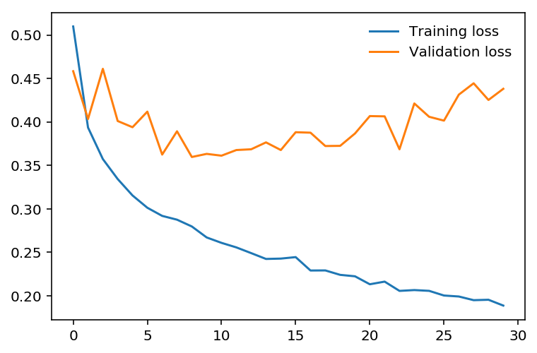
The network learns the training set better and better, resulting in lower training losses. However, it starts having problems generalizing to data outside the training set leading to the validation loss increasing. The ultimate goal of any deep learning model is to make predictions on new data, so we should strive to get the lowest validation loss possible. One option is to use the version of the model with the lowest validation loss, here the one around 8-10 training epochs. This strategy is called early-stopping. In practice, you'd save the model frequently as you're training then later choose the model with the lowest validation loss.

The most common method to reduce overfitting (outside of early-stopping) is dropout, where we randomly drop input units. This forces the network to share information between weights, increasing it's ability to generalize to new data. Adding dropout in PyTorch is straightforward using the nn.Dropout module.

class Classifier(nn.Module):  # Define neural network class
    def __init__(self):  # Initialize network layers
        super().__init__()  # Initialize parent class
        self.fc1 = nn.Linear(784, 256)  # First fully connected layer
        self.fc2 = nn.Linear(256, 128)  # Second fully connected layer
        self.fc3 = nn.Linear(128, 64)  # Third fully connected layer
        self.fc4 = nn.Linear(64, 10)  # Output layer
        
        # Dropout module with 0.2 drop probability
        self.dropout = nn.Dropout(p=0.2)  # Dropout for regularization
        
    def forward(self, x):
        # make sure input tensor is flattened
        x = x.view(x.shape[0], -1)  # Flatten: (batch, 1, 28, 28) -> (batch, 784)
        
        # Now with dropout
        x = self.dropout(F.relu(self.fc1(x)))  # FC1 -> ReLU -> Dropout
        x = self.dropout(F.relu(self.fc2(x)))  # FC2 -> ReLU -> Dropout
        x = self.dropout(F.relu(self.fc3(x)))  # FC3 -> ReLU -> Dropout
        
        # output so no dropout here
        x = F.log_softmax(self.fc4(x), dim=1)  # FC4 -> LogSoftmax output
        
        return x  # Return output tensor

During training we want to use dropout to prevent overfitting, but during inference we want to use the entire network. So, we need to turn off dropout during validation, testing, and whenever we're using the network to make predictions. To do this, you use model.eval(). This sets the model to evaluation mode where the dropout probability is 0. You can turn dropout back on by setting the model to train mode with model.train(). In general, the pattern for the validation loop will look like this, where you turn off gradients, set the model to evaluation mode, calculate the validation loss and metric, then set the model back to train mode.

# turn off gradients
with torch.no_grad():  # Disable gradient computation
    
    # set model to evaluation mode
    model.eval()  # Set to evaluation mode
    
    # validation pass here
    for images, labels in testloader:  # Loop through test batches
        ...

# set model back to train mode
model.train()  # Set to training mode

Exercise: Add dropout to your model and train it on Fashion-MNIST again. See if you can get a lower validation loss or higher accuracy.

## TODO: Define your model with dropout added

model = Classifier()
criterion = nn.NLLLoss()  # Negative log-likelihood loss
optimizer = optim.Adam(model.parameters(), lr=0.003)  # Adam optimizer

epochs = 15  # Number of training epochs
steps = 0  # Initialize step counter

train_losses, test_losses = [], []  # Initialize lists to track losses
for e in range(epochs):
    running_loss = 0  # Initialize loss accumulator
    for images, labels in trainloader:  # Loop through training batches
        
        optimizer.zero_grad()  # Clear previous gradients
        
        log_ps = model(images)
        loss = criterion(log_ps, labels)  # Calculate loss
        loss.backward()  # Backpropagate gradients
        optimizer.step()  # Update model weights
        
        running_loss += loss.item()
        
    else:
        test_loss = 0  # Reset test loss
        accuracy = 0  # Reset accuracy counter
        
        # Turn off gradients for validation, saves memory and computations
        with torch.no_grad():  # Disable gradient computation
            model.eval()  # Set to evaluation mode
            for images, labels in testloader:  # Loop through test batches
                log_ps = model(images)  # Forward pass: get log-probabilities
                test_loss += criterion(log_ps, labels)
                
                ps = torch.exp(log_ps)  # Convert log-probs to probabilities
                top_p, top_class = ps.topk(1, dim=1)  # Get top prediction
                equals = top_class == labels.view(*top_class.shape)  # Compare predictions to actual labels
                accuracy += torch.mean(equals.type(torch.FloatTensor))
        
        model.train()  # Set to training mode
        
        train_losses.append(running_loss/len(trainloader))  # Save average training loss
        test_losses.append(test_loss/len(testloader))  # Save average test loss

        print("Epoch: {}/{}.. ".format(e+1, epochs),
              "Training Loss: {:.3f}.. ".format(train_losses[-1]),
              "Test Loss: {:.3f}.. ".format(test_losses[-1]),
              "Test Accuracy: {:.3f}".format(accuracy/len(testloader)))

%matplotlib inline  # Enable inline plotting in notebook
%config InlineBackend.figure_format = 'retina'

import matplotlib.pyplot as plt  # Import matplotlib for visualization

plt.plot(train_losses, label='Training loss')  # Plot training loss curve
plt.plot(test_losses, label='Validation loss')  # Plot test/validation loss curve
plt.legend(frameon=False)  # Add legend to plot

Inference

Now that the model is trained, we can use it for inference. We've done this before, but now we need to remember to set the model in inference mode with model.eval(). You'll also want to turn off autograd with the torch.no_grad() context.

# Import helper module (should be in the repo)
import helper  # Import helper visualization functions

# Test out your network!

model.eval()  # Set to evaluation mode

dataiter = iter(testloader)
images, labels = next(dataiter)  # Get one batch of images and labels
img = images[0]
# Convert 2D image to 1D vector
img = img.view(1, 784)

# Calculate the class probabilities (softmax) for img
with torch.no_grad():  # Disable gradient computation
    output = model.forward(img)

ps = torch.exp(output)  # Convert log-probs to probabilities

# Plot the image and probabilities
helper.view_classify(img.view(1, 28, 28), ps, version='Fashion')  # Display classification result

Next Up!

In the next part, I'll show you how to save your trained models. In general, you won't want to train a model everytime you need it. Instead, you'll train once, save it, then load the model when you want to train more or use if for inference.